

I’ve been learning about neural networks and I wanted to take you along with me building a neural network to generate new names that seem real but don’t exist yet. The neural network will be trained on a list of about 32,000 names that is publicly available on the internet. It will then be able to output new names based on its training data. That is the goal and it’s not going to be easy so this is part 1 of the series.
my goal is to start generating names using bigram frequency, and then in part 2 we will start building a single layer neural network to do the same thing.
So where do we begin?
Let’s take a look at the dataset we are working with
words = open('names.txt', 'r').read().splitlines()
words[:10]

[’emma’,
 ‘olivia’,
 ‘ava’,
 ‘isabella’,
 ‘sophia’,
 ‘charlotte’,
 ‘mia’,
 ‘amelia’,
 ‘harper’,
 ‘evelyn’]
pretty simple, one name per line, lets get some more info next
len(words)
32033

min(len(w) for w in words)
2

max(len(w) for w in words)
15
okay cool so there is about 32,000 names in the training data, the shortest name is 2 letters long and the longest name is 15 letters long.
to outline my initial approach to the problem of generating new names based on the training data is the following: we can deterministically figure out the probability of one letter coming after another by going through the entire dataset, keeping track of all the bigrams (two letter words combos such as ‘eg’ or ‘va’) and then determine probabilities of each bigram occurring, and then using those probabilities make a guess at what letter is likely to come next given a letter, and use that to build up full names by continuously generating the next letter based on the previous. So we will only be looking one letter ahead for now.
if that’s a bit confusing dont worry, lets get into it step by step.
so firstly lets loop through all the words in the list of words, and for each word we use a clever method called zip we allows us to iterate through every bigram in all the names in the text file. additionally for every name we iterate through we add special characters to denote the start and end of each name. this will help us later on in figuring out the probabilities of a word starting/ending with a letter.
b = {}
for w in words:
    chs = ['<S>'] + list(w) + ['<E>']
    for ch1, ch2 in zip(chs, chs[1:]):
        bigram = (ch1, ch2)
        b[bigram] = b.get(bigram, 0) + 1
        #print(ch1, ch2)
sorted(b.items(), key = lambda kv: -kv[1])

[(('n', '<E>'), 6763),
 (('a', '<E>'), 6640),
 (('a', 'n'), 5438),
 (('<S>', 'a'), 4410),
 (('e', '<E>'), 3983),
 (('a', 'r'), 3264),
 (('e', 'l'), 3248),
 (('r', 'i'), 3033),
 (('n', 'a'), 2977),
...]
if you can’t decipher the output above, this is what is happening: we maintain a dictionary of all the bigrams and their frequencies then we break each word into it’s bigrams and increment it’s corresponding count in the map. after we’ve looped through all the words we sort the map, in this case the most common bigram is (‘n’, ‘<E>’) indicating ‘n’ followed by the name ending.
to make the code very clear the flow for the name “emma” would be processed like this: “emma” → “<S>emma<E>” → [(“<S>”, “e”), (“e”, “m”),…] and so on for all the bigrams in “emma”.
so this works but it’s not very efficient or extendable. ideally what we want is a 2D array/matrix that will store the counts for each possible bigram combo where we have ‘a’ to ‘z’ down the x-axis and ‘a’ to ‘z’ along the y-axis as well as a row and column for ‘.’. we would then easily be able to find the probably of “a” coming after “n” by finding “a” on the x-axis and “n” on the y-axis and lining them up. again if this doesn’t make sense, just scroll down a bit to see the final matrix we come up with.
first to make our lives easier lets start using PyTorch instead of default Python code.
another note: instead of keeping track of <S> and <E> for the start and end we will instead replace them both with a “.” - this will make our matrix much easier to read. a future optimisation would preferably use different tokens for start vs end but lets keep our lives simple for now.
we will import Torch and create a 27x27. that is 26 letters + the “.” to indicate either start/end.
import torch
N = torch.zeros((27,27), dtype = torch.int32)
this just create a 2D array with all counts starting at 0.
given that our matrix works in numbers(or indexes) and not letters we will need a method to convert letters to indices into the matrix.
chars = sorted(list(set(''.join(words))))
stoi = {s:i+1 for i,s in enumerate(chars)}
stoi['.'] = 0
itos = {i:s for s,i in stoi.items()}

stoi
{'a': 1, 'b': 2, 'c': 3,'d': 4,'e': 5,'f': 6,'g': 7,'h': 8,'i': 9,'j': 10,'k': 11,
'l': 12, 'm': 13,'n': 14,'o': 15,'p': 16,'q': 17,'r': 18,'s': 19,'t': 20, 'u': 21,
 'v': 22, 'w': 23, 'x': 24, 'y': 25, 'z': 26,'.': 0}
stoi{} converts the letters into numbers and the itos{} converts the numbers back into their corresponding letters. above is what stoi map looks like.
next we can loop through all the bigrams again but this time we will be adding the counts to our 2D array/matrix.
for w in words:
    chs = ['.'] + list(w) + ['.']
    for ch1, ch2 in zip(chs, chs[1:]):
        ix1 = stoi[ch1]
        ix2 = stoi[ch2]
        N[ix1, ix2] += 1
once we have done that lets visualise our progress so far.
import matplotlib.pyplot as plt
%matplotlib inline

plt.figure(figsize=(16,16))
plt.imshow(N, cmap='Blues')
for i in range(27):
    for j in range(27):
        chstr = itos[i] + itos[j]
        plt.text(j, i, chstr, ha="center", va="bottom", color='gray')
        plt.text(j, i, N[i,j].item(), ha="center", va="top", color='gray')
plt.axis('off')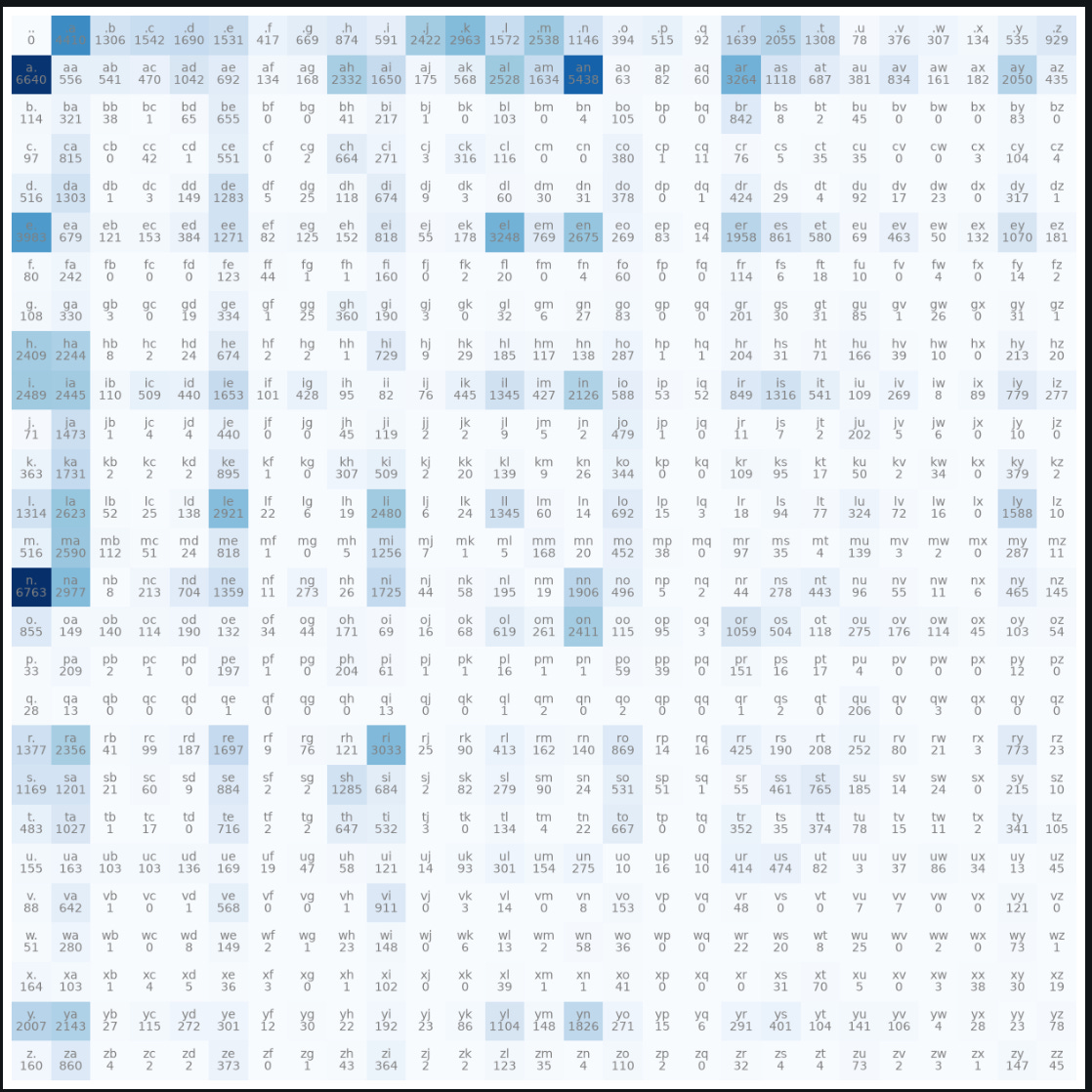
now we have a table with every bigram count from our training data. for example the entry “zh” = 43 tells us that the string “zh” occurs 43 times in all the names in the training data. also “.g” = 669 implies 669 names start with ‘g’ and lastly “x.” = 164 implies that 164 names end with x.
so now lets take the second row for example, this is the row for ‘b’, so if we want to figure out the most likely next letter in the name given the current letter we are looking at is ‘b’ this is the row that will help us do that.
we can sum the row’s counts for each entry in b’s row and then divide each entries count by the row’s sum to determine the probability of that specific letter coming after ‘b’ in a name.
in other words we are normalising the row. the values in the row after dividing will now sum to 1.
lets do that for just row ‘b’ first:
N[2]
tensor([114, 321,  38,   1,  65, 655,   0,   0,  41, 217,   1,   0, 103,   0,
          4, 105,   0,   0, 842,   8,   2,  45,   0,   0,   0,  83,   0],
       dtype=torch.int32)
p = N[2].float()
p = p / p.sum()
p
tensor([0.0000, 0.1377, 0.0408, 0.0481, 0.0528, 0.0478, 0.0130, 0.0209, 0.0273,
        0.0184, 0.0756, 0.0925, 0.0491, 0.0792, 0.0358, 0.0123, 0.0161, 0.0029,
        0.0512, 0.0642, 0.0408, 0.0024, 0.0117, 0.0096, 0.0042, 0.0167, 0.0290])
firstly we just grab the ‘b’ row from the matrix, we then convert the values to floats so they can have decimal points. Once we have done that we can take each entry in the row and divide it by the sum of the row(normalise it). that gives us the p tensor. this contains the probabilities of each letter occurring next given we have a ‘b’ right now as the current letter. example: p[4] gives us the probability that ‘c’ comes after ‘b’ based on the names we have seen in the training data set. 0.0481 implies there is about a 5% chance that ‘c’ would be the next letter after ‘b’.
now given a single rows probabilities how do we choose the next letter based on those probabilities? this is where the multinomial comes in…
p = tensor([0.0000, 0.1377, 0.0408, 0.0481, 0.0528, 0.0478, 0.0130, 0.0209, 0.0273,
        0.0184, 0.0756, 0.0925, 0.0491, 0.0792, 0.0358, 0.0123, 0.0161, 0.0029,
        0.0512, 0.0642, 0.0408, 0.0024, 0.0117, 0.0096, 0.0042, 0.0167, 0.0290])
from earlier^^^

ix = torch.multinomial(p, num_samples=1, replacement=True).item()
itos[ix]
'd'
the above code uses the probabilities above to choose a number between 1 and 27, each with a probability of being chosen given above in the tensor p. the numbers it chooses correspond to the index of the letter it determines is likely to come next.
we then convert that chosen index into a string using the map we created earlier and the output is ‘d’. based on the probabilities, and relative frequency from our training data ‘d’ had a 5% chance of being after ‘b’. if we kept sampling using the multinomial we would probably get a different letter each time, it does not pick the most likely next letter, it picks a letter based on it’s probability to be picked which is what is stored in tensor p.
to sample an entire word we would run the above code again and again. so we would generate ‘b’ lets say as the first letter using the top row of our table above(since the top row corresponds to probabilities of words starting with that given letter) and then we would refer to the row corresponding to ‘b’ to generate the next letter and so on until we generate a ‘.’ which means the end of the name.
lets do this now - first lets turn the entire matrix we generated above into probabilities (in other words normalise every row) so we dont need to normalise each row every time we sample. you’ll observe now that each row in the matrix below sums to 1.
P = N.float()
P /=P.sum(1, keepdims=True)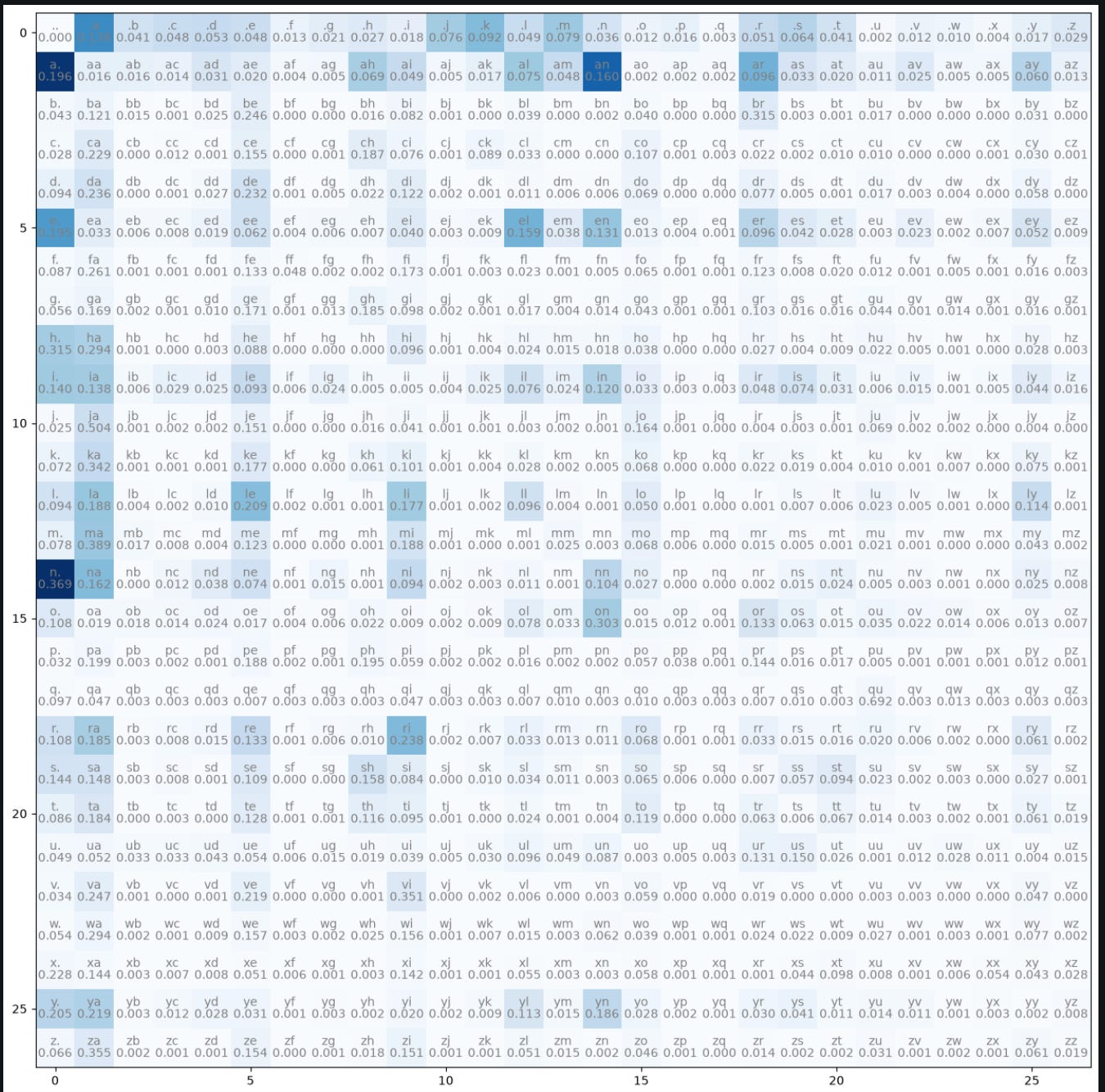
now that we have our probability matrix we can start sampling from it. lets generate 5 names:
for i in range(5):
    ix = 0
    out = []
    while True:
        p = P[ix]
        ix = torch.multinomial(p, num_samples=1, replacement=True).item()
        out.append(itos[ix])
        if ix == 0:
            break
    print(''.join(out))

cexze.
momasurailezitynn.
konimittain.
llayn.
ka.
read through the code and convince yourself that this is using the probability matrix above to continuously generate letters based on the previous letter until we reach a ‘.’ which means the word has ended. remember given any letter there is always a chance the next character is a ‘.’ which implies the end of a name. refer to the first column of the above matrix for those probabilities.
fair enough that worked but did it really?
the names we generated still look pretty random, how can we prove that we did “train” this network on the 32,000 names in the text file.
well lets say we add 10000 to every probability in the P matrix above, in other words make every letter just as likely as the next for every letter, here is the output:
for i in range(4):
    ix = 0
    out = []
    while True:
        p = P[ix] + 10000
        ix = torch.multinomial(p, num_samples=1, replacement=True).item()
        out.append(itos[ix])
        if ix == 0:
            break
    print(''.join(out))

zoglkurkicqzktyhwmvmzimjttainrlkfukzkktda.
sfcxvpubjtbhrmgotzx.
iczixqctvujkwptedogkkjemkmmsidguenkbvgynywftbspmhwcivgbvtahlvsu.
dsdxxblnwglhpyiw.
as you can see the output is pretty garbage compared to what we had earlier. i call that progress!!!
and that as far as we are going to go today…
as a sneak peek of what we will do in part 2…we need a way of calculating how “good” the output is compared to what we would actually like it to output. we will be using something called the negative log likelihood for this.
this will help us adjust the weights and biases of our neural network. what we end up doing with the neural net is basically updating the matrix P’s probabilities to be as accurate as possible but instead of counting the frequencies of bigrams we feed in training data and adjusts parameters which adjusts the values stored in P.
for now dont worry about that, if you’re excited for part 2 the best thing you can do now is understand what we did today back to front, implement it yourself, try the exercise below. you can use your own .txt file of names or any training data. use your llm of choice to explain anything I missed or glossed over. get your code working like mine and I promise you will double your level of understanding.
next up → real neural networks!
an exercise for the readers at home, try to extend this program but instead of using bi-grams I want you to use tri-grams. In other words, find the next most likely letter based on the TWO preceding letters instead of just the previous letter.
references:
Interesting, love your content Tomdev